Topographic Contour Lines

Topographic contour lines of Colorado drawn in a Google Earth satellite image.

Elevation (MSL)

Orange = 5500 ft

Pink = 7500 ft

Purple = 8500 ft

Yellow = 9500 ft

Blue = 10500 ft


For examples of other types of maps please follow this link. 

Rocks & Soils

IGNEOUS

Taken from the following website: http://skywalker.cochise.edu/wellerr/GLG101/GLG101-igneous-rocks.htm

“Pegmatite is very coarsely crystallized.  Some of the largest crystals in the world have 
been found in pegmatites.  Pegmatites often have the same mineral composition of granites with large crystals of mica and feldspar.  Gem minerals, such as tourmaline and beryl are found in pegmatites.”
 

Pic: Shkatulka pegmatite

Geographic Area of Abundance: Russia

Link: http://www.mindat.org/min-7291.html

METAMORPHIC

Taken from the following website: http://www.rocksandminerals4u.com/marble.html

“Marble is a metamorphic rock that comes from metamorphosed limestone or dolomite. Limestone is mostly calcite or calcium carbonate, CaCO₃. Dolomite CaMg(CO₃)₂ is related to limestone but is rich in magnesium. Marble has a uniform texture (non-foliated).”

Pic: Gray Marble

Geographic Area of Abundance: China, Italy, United States, India and Greece, among others

Link: http://geology.com/rocks/marble.shtml

SEDIMENTARY

Taken from the following website: http://geology.com/rocks/breccia.shtml

“Breccia is a term most often used for clastic sedimentary rocks that are composed of large angular fragments (over two millimeters in diameter). The spaces between the large angular fragments can be filled with a matrix of smaller particles or a mineral cement that binds the rock together.“

Pic: Chert Breccia

Geographic Area of Abundance: Western Australia

Link: http://outbackmining.com/chert_Breccia.htm

http://geology.com/rocks/breccia.shtml

12 SOIL ORDERS OF THE WORLD: found here.

SOIL TEXTURE DIAGRAM

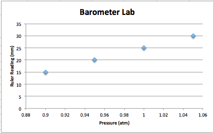
Barometer Lab

1 atm = 760 mmHg1.00 in = 2.54 cm The device made and used in this lab is pictured above. A table with the information gathered is presented below. As the pressure goes up in a system, the ruler reading goes up. As the pressure in the system lowers, the ruler reading goes down. This relationship is shown in the graph below. 

The Life of Ua Jua

This is a blog of the life of a sunflower that I am growing this semester. I will be regularly updating the post the rest of the semester until it's time to plant it. It took one week for the seed to sprout. The sprout started bending towards the sun throughout the day. Once it got too long, it wouldn't stay up. I tied it to a straw for more support.

Day               Height (inches)
1                     0.0
7                     0.5
9                     2.5
11                   4.5
18                   8.0

 

 

Lakes Environmental Windrose Plot Lab

WRPlot Freeware from Lakes Environmental was used in this lab to determine wind patterns at a specified location. For this lab, SCRAM data from the EPA's website was used; specifically data from Wisconsin General Mitchell International Airport in Milwaukee, Wisconsin in the year 1984. Each windrose plot shows the direction the wind is coming from. Google Earth was used to obtain a satellite image of the airport. A windrose plot of the full year was overlaid on the image, (see first image). The other images included below are windrose plots of specific seasons throughout the year as follows: Summer, Fall, Winter, Spring, Year-round.  

Windrose plots allow data to be presented in a way that evaluates changes in wind velocity at a specific station/location. Most of the stronger wind readings were recorded as coming from the Southwest quadrant. In the Spring a majority of the stronger wind readings came from the North/Northeast. 

 

Summer                                                         Fall 

Winter                                                        Spring 

  

Year-Round 1984

Sun Trajectory Lab

Data Recorded for Sun Trajectory Lab- 1/25/14
Time of Day	Length of Shadow (in.)	Height of Pole (in.)	Direction of Shadow	Angle of Sun  (degrees)
7:30 am	22	6.5	West	16.5
9:00 am	6	6.5	Northwest	47
12 noon	0.5	6.5	North	85.5
3:00 pm	7	6.5	Northeast	43
6:00 pm	22	6.5	East	16.5

The purpose of this lab is to determine the trajectory of the sun based on the height of a pole (in this case we used a pencil), the length of its shadow, and the direction the shadow is cast. A pencil was set up on campus and the height was measured. The length of the shadow and its direction were then measured at the times listed in the table above over a 24 hr period. All this data was used to draw the shadow trajectory image above. SunCalc was used as another visual aid to better understand the trajectory of the sun.